Day 2 Lectures

Author

AJ Smit

1 This is a heading

This is the same comment that I hash out inside the code block: load the tidyverse library

# load the tidyverse library
library(tidyverse)

mean(1, 2, 3)

[1] 1

1.1 Numeric data

# Create a vector of the number of pets owned by each household
num_rats <- c(0, 1, 2, 2, 3, 1, 4, 0, 2, 1, 2, 2, 0, 3, 2, 1, 1, 4, 2, 0)
num_rats

 [1] 0 1 2 2 3 1 4 0 2 1 2 2 0 3 2 1 1 4 2 0

class(num_rats)

[1] "numeric"

num_rats_int <- as.integer(num_rats) # coercion
num_rats_int

 [1] 0 1 2 2 3 1 4 0 2 1 2 2 0 3 2 1 1 4 2 0

class(num_rats_int)

[1] "integer"

pies <- pi * seq(1:5)
pies

[1]  3.141593  6.283185  9.424778 12.566371 15.707963

class(pies)

[1] "numeric"

as.integer(pies)

[1]  3  6  9 12 15

round(pies, 2)

[1]  3.14  6.28  9.42 12.57 15.71

The as.integer() function does not care about rouning, for example:

as.integer(round(pies, 2))

[1]  3  6  9 12 15

set.seed(13)
# Generate a vector of 50 normally distributed temperature values
temp_data <- round(rnorm(n = 50, mean = 15, sd = 3), 2)
# temp_data <- rnorm(n = 50, mean = 15, sd = 3)
temp_data

 [1] 16.66 14.16 20.33 15.56 18.43 16.25 18.69 15.71 13.90 18.32 11.72 16.39
[13] 10.92  9.43 13.68 14.42 19.19 15.30 14.66 17.11 15.79 20.51 16.07 11.86
[25] 16.86 15.45 10.62  8.92 11.83 12.82 14.98 17.54 13.85 13.42 14.18 13.18
[37] 14.00 14.28 12.41 12.46 15.30 19.77 16.70 19.84 13.59 12.82 11.93  9.19
[49] 15.83 19.23

length(temp_data)

[1] 50

mean(temp_data)

[1] 14.9212

sd(temp_data)

[1] 2.92563

class(temp_data)

[1] "numeric"

names <- c("Fluffy", "Jesse")
names <- c('Fluffy', 'Jesse')
class(names)

[1] "character"

1.2 Factor data

# Generate a vector of vegetation types

vegetation <- sample(c("grassland", "forest", "wetland"), size = 50, replace = TRUE)

# View the vegetation data
vegetation

 [1] "forest"    "wetland"   "grassland" "grassland" "grassland" "wetland"  
 [7] "grassland" "wetland"   "grassland" "grassland" "wetland"   "forest"   
[13] "wetland"   "forest"    "forest"    "grassland" "wetland"   "grassland"
[19] "grassland" "grassland" "forest"    "wetland"   "grassland" "forest"   
[25] "grassland" "forest"    "forest"    "grassland" "forest"    "grassland"
[31] "grassland" "wetland"   "wetland"   "grassland" "grassland" "forest"   
[37] "wetland"   "grassland" "forest"    "forest"    "grassland" "grassland"
[43] "forest"    "forest"    "grassland" "forest"    "grassland" "wetland"  
[49] "wetland"   "forest"

class(vegetation)

[1] "character"

veg_fact <- as.factor(vegetation)
class(veg_fact)

[1] "factor"

1.3 Ordered factors

# Vector of ordinal data representing the successional stage of a forest
coffee <- c("Small", "Tall", "Venti", "Grande", "Ginormous")
class(coffee)

[1] "character"

# Convert to ordered factor
coffee <- factor(coffee, ordered = TRUE,
                 levels = c("Small", "Tall", "Venti",
                            "Grande", "Ginormous"))
coffee

[1] Small     Tall      Venti     Grande    Ginormous
Levels: Small < Tall < Venti < Grande < Ginormous

class(coffee)

[1] "ordered" "factor"

1.4 Logical data

# Generate a vector of 1s and 0s to represent the presence
# or absence of a species in different ecological sites
species_presence <- sample(c(0, 1), 10,
                           replace = TRUE)
class(species_presence)

[1] "numeric"

species_presence_logi <- as.logical(species_presence)
class(species_presence_logi)

[1] "logical"

1.5 Dates

my_time <- as.POSIXct("2022-03-10 12:34:56")
class(my_time)

[1] "POSIXct" "POSIXt"

1.6 Missing values

# Set the length of the sequence
n <- 100

# Generate a sequence of random normal numbers with
# mean 0 and standard deviation 1
data <- rnorm(n, mean = 0, sd = 1)

# Randomly assign 5% of the values as missing
missing_indices <- sample(1:n, size = round(0.05*n))
data[missing_indices] <- NA
length(data)

[1] 100

mean(data, na.rm = TRUE)

[1] -0.1332528

length(data)

[1] 100

data_sans_na <- na.omit(data)
length(data_sans_na)

[1] 95

1.7 Matrices (plural) and a matric (singular)

# create a numeric matrix
my_matrix_1 <- matrix(1:6, nrow = 2, ncol = 3,
                    byrow = FALSE)

my_matrix_2 <- matrix(1:6, nrow = 2, ncol = 3,
                    byrow = TRUE)

# print the matrix
my_matrix_1

     [,1] [,2] [,3]
[1,]    1    3    5
[2,]    2    4    6

my_matrix_2

     [,1] [,2] [,3]
[1,]    1    2    3
[2,]    4    5    6

dim(my_matrix_1)

[1] 2 3

mat <- matrix(rnorm(n = 15, mean = 0, sd = 1),
              nrow = 5, ncol = 3)
mat <- round(mat, 2)
dim(mat)

[1] 5 3

ncol(mat)

[1] 3

nrow(mat)

[1] 5

# coerce the matrixto a vector
# 2D to 1D
vect <- as.vector(mat)
vect

 [1] -1.04  0.82  1.00  0.43  0.47 -1.10  0.61  0.02  0.74  1.25 -0.73 -0.07
[13]  1.03  0.82 -0.45

length(vect)

[1] 15

mat

      [,1]  [,2]  [,3]
[1,] -1.04 -1.10 -0.73
[2,]  0.82  0.61 -0.07
[3,]  1.00  0.02  1.03
[4,]  0.43  0.74  0.82
[5,]  0.47  1.25 -0.45

mat[2, ]

[1]  0.82  0.61 -0.07

mat[5, c(1, 3)]

[1]  0.47 -0.45

1.8 Arrays

# create a 2-dimensional array
my_array <- array(1:27, dim = c(3, 3, 3))

# print the array
my_array

, , 1

     [,1] [,2] [,3]
[1,]    1    4    7
[2,]    2    5    8
[3,]    3    6    9

, , 2

     [,1] [,2] [,3]
[1,]   10   13   16
[2,]   11   14   17
[3,]   12   15   18

, , 3

     [,1] [,2] [,3]
[1,]   19   22   25
[2,]   20   23   26
[3,]   21   24   27

dim(my_array)

[1] 3 3 3

my_array[2, 2, 2]

[1] 14

# square bracket notation:
# [row, column, depth]
my_array[2, 3, 3]

[1] 26

as.vector(my_array)

 [1]  1  2  3  4  5  6  7  8  9 10 11 12 13 14 15 16 17 18 19 20 21 22 23 24 25
[26] 26 27

1.9 Making a data.frame

# Create a vector of dates
dates <- as.Date(c("2022-01-01", "2022-01-02", "2022-01-03",
                   "2022-01-04", "2022-01-05"))

# Create a vector of numeric data
numeric_data <- rnorm(n = 5, mean = 0, sd = 1)

# Create a vector of categorical data
categorical_data <- c("A", "B", "C", "A", "B")

# Combine the vectors into a data.frame
my_dataframe <- data.frame(day = dates,
                           number = numeric_data,
                           category = categorical_data)

# Print the dataframe
my_dataframe

         day     number category
1 2022-01-01  1.1059215        A
2 2022-01-02  1.2593616        B
3 2022-01-03 -0.6061951        C
4 2022-01-04 -1.4083780        A
5 2022-01-05  1.6957718        B

class(my_dataframe)

[1] "data.frame"

colnames(my_dataframe)

[1] "day"      "number"   "category"

rownames(my_dataframe)

[1] "1" "2" "3" "4" "5"

dim(my_dataframe)

[1] 5 3

str(my_dataframe)

'data.frame':   5 obs. of  3 variables:
 $ day     : Date, format: "2022-01-01" "2022-01-02" ...
 $ number  : num  1.106 1.259 -0.606 -1.408 1.696
 $ category: chr  "A" "B" "C" "A" ...

mean(my_dataframe$number)

[1] 0.4092964

range(my_dataframe$day)

[1] "2022-01-01" "2022-01-05"

summary(my_dataframe)

      day                 number          category        
 Min.   :2022-01-01   Min.   :-1.4084   Length:5          
 1st Qu.:2022-01-02   1st Qu.:-0.6062   Class :character  
 Median :2022-01-03   Median : 1.1059   Mode  :character  
 Mean   :2022-01-03   Mean   : 0.4093                     
 3rd Qu.:2022-01-04   3rd Qu.: 1.2594                     
 Max.   :2022-01-05   Max.   : 1.6958

glimpse(my_dataframe)

Rows: 5
Columns: 3
$ day      <date> 2022-01-01, 2022-01-02, 2022-01-03, 2022-01-04, 2022-01-05
$ number   <dbl> 1.1059215, 1.2593616, -0.6061951, -1.4083780, 1.6957718
$ category <chr> "A", "B", "C", "A", "B"

my_tibble <- as_tibble(my_dataframe)
class(my_tibble)

[1] "tbl_df"     "tbl"        "data.frame"

my_tibble

# A tibble: 5 × 3
  day        number category
  <date>      <dbl> <chr>   
1 2022-01-01  1.11  A       
2 2022-01-02  1.26  B       
3 2022-01-03 -0.606 C       
4 2022-01-04 -1.41  A       
5 2022-01-05  1.70  B

1.10 Exercise in frustration

read_csv("../data/SAMOS/other_data/SACTN_SAWS.csv") |> 
  mutate(month = as.integer(month(date, label = FALSE))) |> 
  group_by(site) |> 
  mutate(temp_y = mean(temp, na.rm = TRUE)) |> 
  group_by(site, month) |> 
  summarise(temp_m = mean(temp, na.rm = TRUE),
            temp_y = mean(temp_y)) |> 
  ggplot(aes(x = month)) +
    geom_line(aes(y = temp_y), colour = "red") +
    geom_line(aes(y = temp_m)) +
    scale_x_continuous(breaks = c(3, 6, 9, 12)) +
    facet_wrap(~site)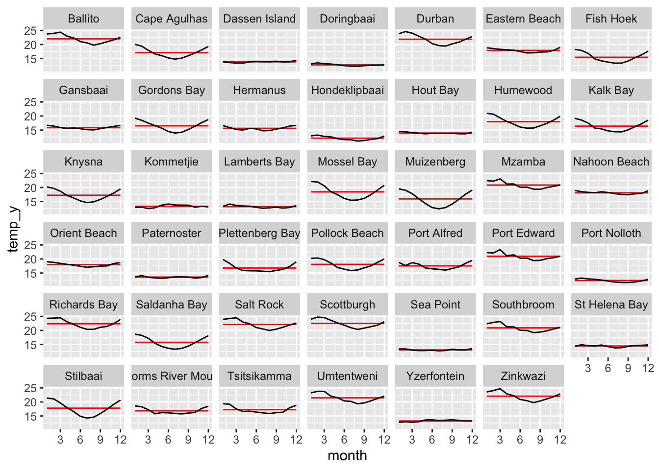

1.11 Reading in data into R

For this exercise, we will use the laminaria.csv file. It is located in the data/SAMOS/other_data folder.

laminaria <- read_csv("../data/SAMOS/other_data/laminaria.csv")

laminaria

# A tibble: 140 × 12
   region site          Ind blade_weight blade_length blade_thickness stipe_mass
   <chr>  <chr>       <dbl>        <dbl>        <dbl>           <dbl>      <dbl>
 1 WC     Kommetjie       2         1.9           160            2          1.5 
 2 WC     Kommetjie       3         1.5           120            1.4        2.25
 3 WC     Kommetjie       4         0.55          110            1.5        1.15
 4 WC     Kommetjie       5         1             159            1.5        2.6 
 5 WC     Kommetjie       6         2.3           149            2         NA   
 6 WC     Kommetjie       7         1.6           107            1.75       2.9 
 7 WC     Kommetjie       8         0.65          104            2          0.75
 8 WC     Kommetjie      10         0.95          111            1.25       1.6 
 9 WC     Kommetjie      11         2.3           178            2.5        4.2 
10 FB     Bordjiesti…     1         1.75          145            1          0.75
# ℹ 130 more rows
# ℹ 5 more variables: stipe_length <dbl>, stipe_diameter <dbl>, digits <dbl>,
#   thallus_mass <dbl>, total_length <dbl>

head(laminaria, 7)

# A tibble: 7 × 12
  region site        Ind blade_weight blade_length blade_thickness stipe_mass
  <chr>  <chr>     <dbl>        <dbl>        <dbl>           <dbl>      <dbl>
1 WC     Kommetjie     2         1.9           160            2          1.5 
2 WC     Kommetjie     3         1.5           120            1.4        2.25
3 WC     Kommetjie     4         0.55          110            1.5        1.15
4 WC     Kommetjie     5         1             159            1.5        2.6 
5 WC     Kommetjie     6         2.3           149            2         NA   
6 WC     Kommetjie     7         1.6           107            1.75       2.9 
7 WC     Kommetjie     8         0.65          104            2          0.75
# ℹ 5 more variables: stipe_length <dbl>, stipe_diameter <dbl>, digits <dbl>,
#   thallus_mass <dbl>, total_length <dbl>

tail(laminaria, 2)

# A tibble: 2 × 12
  region site         Ind blade_weight blade_length blade_thickness stipe_mass
  <chr>  <chr>      <dbl>        <dbl>        <dbl>           <dbl>      <dbl>
1 WC     Rocky Bank    12          2.1          194             1.4       3.75
2 WC     Rocky Bank    13          1.3          160             1.9       2.45
# ℹ 5 more variables: stipe_length <dbl>, stipe_diameter <dbl>, digits <dbl>,
#   thallus_mass <dbl>, total_length <dbl>

summary(laminaria)

    region              site                Ind          blade_weight  
 Length:140         Length:140         Min.   : 1.000   Min.   :0.125  
 Class :character   Class :character   1st Qu.: 4.000   1st Qu.:1.130  
 Mode  :character   Mode  :character   Median : 6.500   Median :1.700  
                                       Mean   : 6.586   Mean   :1.700  
                                       3rd Qu.:10.000   3rd Qu.:2.250  
                                       Max.   :13.000   Max.   :3.800  
                                                                       
  blade_length   blade_thickness   stipe_mass      stipe_length  
 Min.   :100.0   Min.   :0.100   Min.   :0.1250   Min.   : 34.0  
 1st Qu.:121.0   1st Qu.:1.200   1st Qu.:0.6325   1st Qu.: 85.0  
 Median :136.0   Median :1.700   Median :1.1750   Median :109.0  
 Mean   :139.1   Mean   :2.666   Mean   :1.3511   Mean   :111.3  
 3rd Qu.:156.2   3rd Qu.:4.100   3rd Qu.:1.6875   3rd Qu.:134.5  
 Max.   :205.0   Max.   :9.100   Max.   :5.6000   Max.   :224.0  
                                 NA's   :2                       
 stipe_diameter      digits       thallus_mass   total_length  
 Min.   : 2.20   Min.   : 7.00   Min.   : 337   Min.   :145.0  
 1st Qu.:35.88   1st Qu.:12.00   1st Qu.:1750   1st Qu.:209.0  
 Median :42.00   Median :15.00   Median :2650   Median :246.5  
 Mean   :39.21   Mean   :15.77   Mean   :2929   Mean   :249.8  
 3rd Qu.:50.00   3rd Qu.:19.00   3rd Qu.:3662   3rd Qu.:283.2  
 Max.   :76.00   Max.   :29.00   Max.   :9400   Max.   :443.0

glimpse(laminaria)

Rows: 140
Columns: 12
$ region          <chr> "WC", "WC", "WC", "WC", "WC", "WC", "WC", "WC", "WC", …
$ site            <chr> "Kommetjie", "Kommetjie", "Kommetjie", "Kommetjie", "K…
$ Ind             <dbl> 2, 3, 4, 5, 6, 7, 8, 10, 11, 1, 3, 4, 5, 6, 7, 8, 9, 1…
$ blade_weight    <dbl> 1.90, 1.50, 0.55, 1.00, 2.30, 1.60, 0.65, 0.95, 2.30, …
$ blade_length    <dbl> 160, 120, 110, 159, 149, 107, 104, 111, 178, 145, 146,…
$ blade_thickness <dbl> 2.00, 1.40, 1.50, 1.50, 2.00, 1.75, 2.00, 1.25, 2.50, …
$ stipe_mass      <dbl> 1.50, 2.25, 1.15, 2.60, NA, 2.90, 0.75, 1.60, 4.20, 0.…
$ stipe_length    <dbl> 120, 149, 97, 167, 146, 161, 110, 136, 176, 82, 118, 1…
$ stipe_diameter  <dbl> 56.0, 68.5, 69.0, 60.0, 73.0, 63.0, 51.0, 56.0, 76.0, …
$ digits          <dbl> 12, 12, 13, 8, 15, 17, 11, 11, 8, 19, 20, 23, 20, 24, …
$ thallus_mass    <dbl> 3000, 3750, 1700, 3600, 5100, 4500, 1400, 2550, 6500, …
$ total_length    <dbl> 256, 269, 207, 326, 295, 268, 214, 247, 354, 227, 264,…

names(laminaria)

 [1] "region"          "site"            "Ind"             "blade_weight"   
 [5] "blade_length"    "blade_thickness" "stipe_mass"      "stipe_length"   
 [9] "stipe_diameter"  "digits"          "thallus_mass"    "total_length"

library(skimr)
skim(laminaria) # using built-in `iris` data

Name	laminaria
Number of rows	140
Number of columns	12
_______________________
Column type frequency:
character	2
numeric	10
________________________
Group variables	None

Data summary

Variable type: character

skim_variable	n_missing	complete_rate	min	max	empty	n_unique	whitespace
region	0	1	2	2	0	2	0
site	0	1	7	17	0	13	0

Variable type: numeric

skim_variable	n_missing	complete_rate	mean	sd	p0	p25	p50	p75	p100	hist
Ind	0	1.00	6.59	3.52	1.00	4.00	6.50	10.00	13.0	▇▅▇▅▅
blade_weight	0	1.00	1.70	0.77	0.12	1.13	1.70	2.25	3.8	▃▇▇▃▁
blade_length	0	1.00	139.06	23.88	100.00	121.00	136.00	156.25	205.0	▆▇▆▂▁
blade_thickness	0	1.00	2.67	2.14	0.10	1.20	1.70	4.10	9.1	▇▂▂▁▁
stipe_mass	2	0.99	1.35	0.99	0.12	0.63	1.17	1.69	5.6	▇▆▂▁▁
stipe_length	0	1.00	111.26	39.32	34.00	85.00	109.00	134.50	224.0	▃▇▇▃▁
stipe_diameter	0	1.00	39.21	17.97	2.20	35.88	42.00	50.00	76.0	▃▁▇▅▂
digits	0	1.00	15.77	4.80	7.00	12.00	15.00	19.00	29.0	▅▇▇▃▁
thallus_mass	0	1.00	2928.56	1558.51	337.00	1750.00	2650.00	3662.50	9400.0	▆▇▂▁▁
total_length	0	1.00	249.81	55.30	145.00	209.00	246.50	283.25	443.0	▃▇▅▂▁

1.12 Tidyverse sneak peak

# Note: output NOT assigned to an object (no `<-`):
laminaria %>% # Tell R which dataframe you are using ("%>%" == "|>" )
  select(site, total_length) # Select only specific columns

# A tibble: 140 × 2
   site              total_length
   <chr>                    <dbl>
 1 Kommetjie                  256
 2 Kommetjie                  269
 3 Kommetjie                  207
 4 Kommetjie                  326
 5 Kommetjie                  295
 6 Kommetjie                  268
 7 Kommetjie                  214
 8 Kommetjie                  247
 9 Kommetjie                  354
10 Bordjiestif North          227
# ℹ 130 more rows

laminaria %>% 
  select(site, total_length) %>% # Select specific columns first
  slice(56:78)

# A tibble: 23 × 2
   site           total_length
   <chr>                 <dbl>
 1 Miller's Point          215
 2 Miller's Point          186
 3 Miller's Point          179
 4 Miller's Point          268
 5 Miller's Point          194
 6 Miller's Point          207
 7 Miller's Point          167
 8 Baboon Rock             146
 9 Baboon Rock             147
10 Baboon Rock             190
# ℹ 13 more rows

# what does the '56:78' do? Change some numbers and run the code again. What happens?

laminaria %>%
  filter(site == "Kommetjie")

# A tibble: 9 × 12
  region site        Ind blade_weight blade_length blade_thickness stipe_mass
  <chr>  <chr>     <dbl>        <dbl>        <dbl>           <dbl>      <dbl>
1 WC     Kommetjie     2         1.9           160            2          1.5 
2 WC     Kommetjie     3         1.5           120            1.4        2.25
3 WC     Kommetjie     4         0.55          110            1.5        1.15
4 WC     Kommetjie     5         1             159            1.5        2.6 
5 WC     Kommetjie     6         2.3           149            2         NA   
6 WC     Kommetjie     7         1.6           107            1.75       2.9 
7 WC     Kommetjie     8         0.65          104            2          0.75
8 WC     Kommetjie    10         0.95          111            1.25       1.6 
9 WC     Kommetjie    11         2.3           178            2.5        4.2 
# ℹ 5 more variables: stipe_length <dbl>, stipe_diameter <dbl>, digits <dbl>,
#   thallus_mass <dbl>, total_length <dbl>

laminaria |> 
  filter(blade_weight >= 1.5)

# A tibble: 83 × 12
   region site          Ind blade_weight blade_length blade_thickness stipe_mass
   <chr>  <chr>       <dbl>        <dbl>        <dbl>           <dbl>      <dbl>
 1 WC     Kommetjie       2         1.9           160            2          1.5 
 2 WC     Kommetjie       3         1.5           120            1.4        2.25
 3 WC     Kommetjie       6         2.3           149            2         NA   
 4 WC     Kommetjie       7         1.6           107            1.75       2.9 
 5 WC     Kommetjie      11         2.3           178            2.5        4.2 
 6 FB     Bordjiesti…     1         1.75          145            1          0.75
 7 FB     Bordjiesti…     3         2.35          146            1.75       1.25
 8 FB     Bordjiesti…     4         1.7           116            1.25      NA   
 9 FB     Bordjiesti…     6         2.45          136            1          1.95
10 FB     Bordjiesti…     7         2             124            1.25       1.3 
# ℹ 73 more rows
# ℹ 5 more variables: stipe_length <dbl>, stipe_diameter <dbl>, digits <dbl>,
#   thallus_mass <dbl>, total_length <dbl>

lam_kom <- laminaria %>%
  filter(site == "Kommetjie")

laminaria %>% # Tell R which dataset to use
  filter(site == "Kommetjie") %>% # Filter out only records from Kommetjie
  nrow() # Count the number of remaining rows

[1] 9

laminaria %>% # Tell R which dataset to use
  filter(total_length == max(total_length)) # Select row with max total length

# A tibble: 1 × 12
  region site          Ind blade_weight blade_length blade_thickness stipe_mass
  <chr>  <chr>       <dbl>        <dbl>        <dbl>           <dbl>      <dbl>
1 WC     Olifantsbos     4         3.35          205               1          3
# ℹ 5 more variables: stipe_length <dbl>, stipe_diameter <dbl>, digits <dbl>,
#   thallus_mass <dbl>, total_length <dbl>

1.13 Some new functions: summarise, mutate, and group_by

laminaria %>% # Chose the dataframe
  summarise(avg_bld_len = mean(blade_length)) # Calculate mean blade length

# A tibble: 1 × 1
  avg_bld_len
        <dbl>
1        139.

laminaria %>%
  summarise(avg_stp_ln = round(mean(total_length), 1),
            sd_stp_ln = round(sd(total_length), 1))

# A tibble: 1 × 2
  avg_stp_ln sd_stp_ln
       <dbl>     <dbl>
1       250.      55.3

laminaria %>% 
  summarise(avg_stp_ms = mean(stipe_mass, na.rm = TRUE))

# A tibble: 1 × 1
  avg_stp_ms
       <dbl>
1       1.35

res <- laminaria %>%
  group_by(site) %>%
  summarise(var_bl = var(blade_length),
            n_bl = n(),
            sd_bl = sd(blade_length)) %>%
  mutate(se_bl = var_bl / sqrt(n_bl))

res

# A tibble: 13 × 5
   site              var_bl  n_bl sd_bl se_bl
   <chr>              <dbl> <int> <dbl> <dbl>
 1 A-Frame             342.    12  18.5  98.6
 2 Baboon Rock         360.    12  19.0 104. 
 3 Batsata Rock        655.    10  25.6 207. 
 4 Betty's Bay         487.    12  22.1 141. 
 5 Bordjiestif North   283.    10  16.8  89.5
 6 Buffels             207.    12  14.4  59.6
 7 Buffels South       260.    12  16.1  75.1
 8 Kommetjie           798.     9  28.3 266. 
 9 Miller's Point      261.     9  16.1  86.9
10 Olifantsbos         679.    10  26.1 215. 
11 Rocky Bank          568.    11  23.8 171. 
12 Roman Rock          200.    11  14.1  60.3
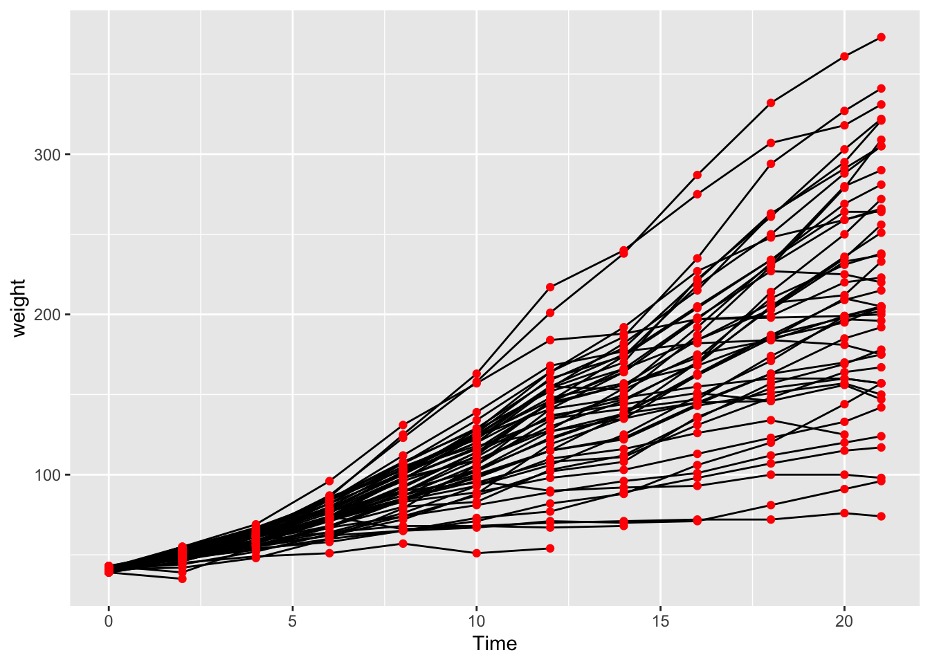
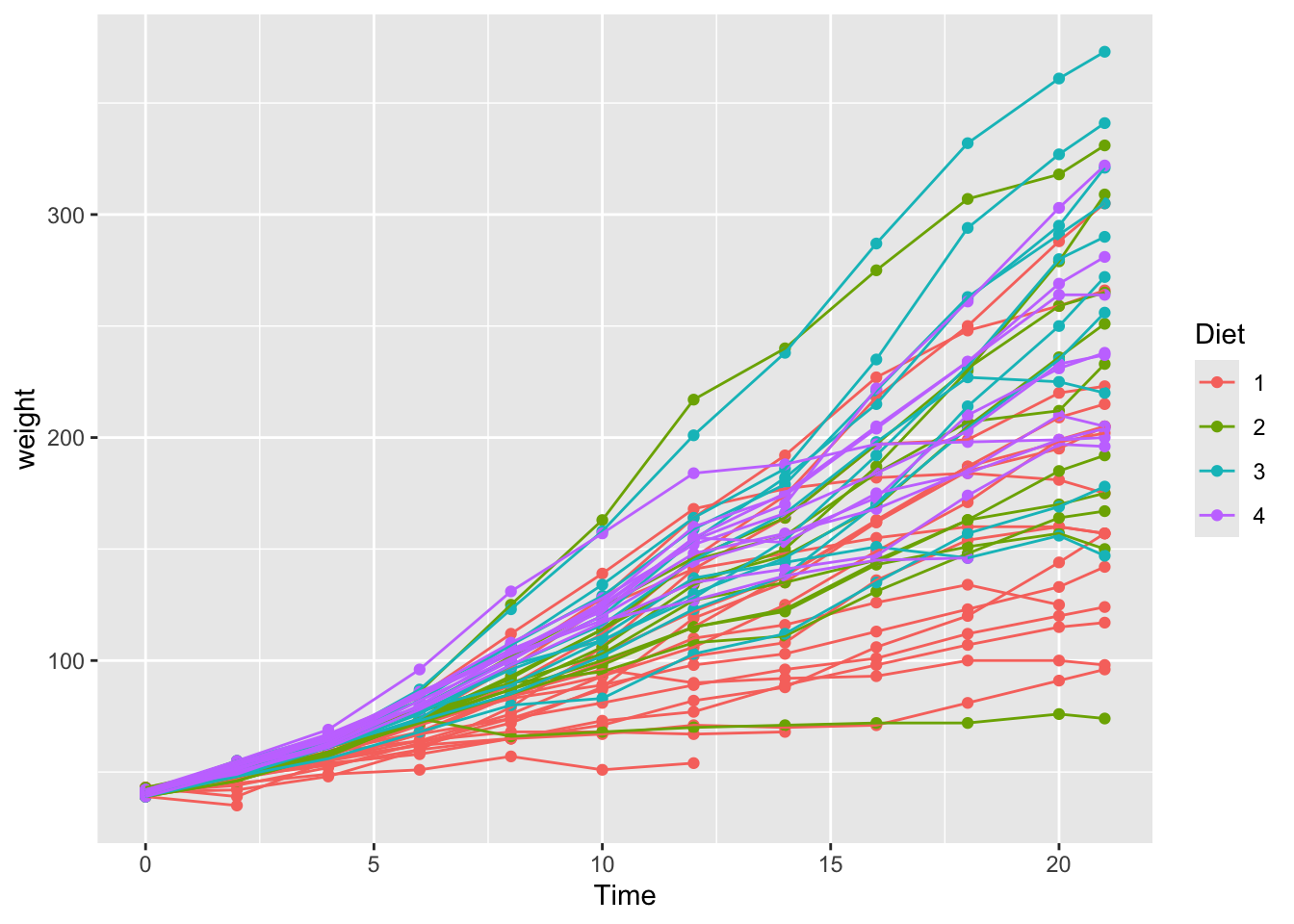
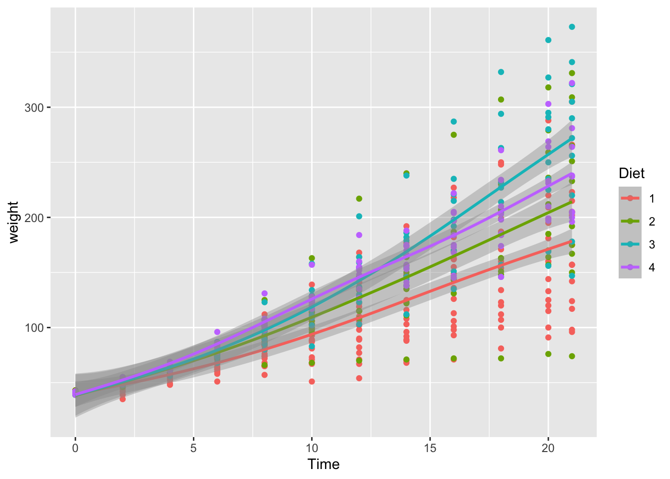
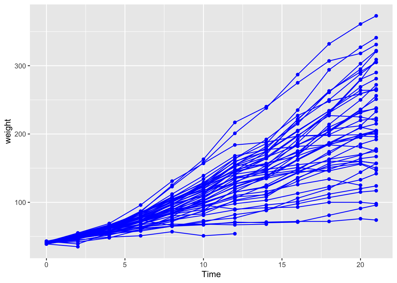
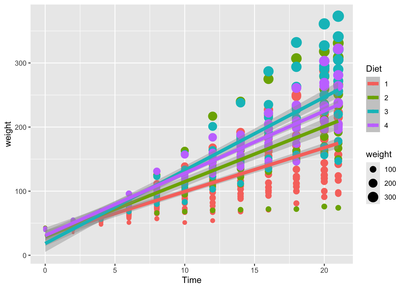
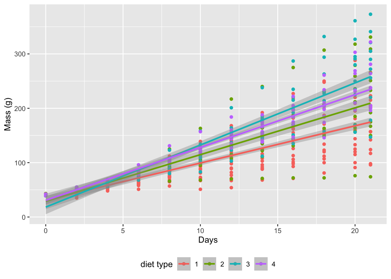
13 Sea Point           471.    10  21.7 149.

write.csv(res, "../data/SAMOS/other_data/laminaria_results.csv")

1.14 Graphics with R

data()

# Load data
ChickWeight <- datasets::ChickWeight

# Create a basic figure
ggplot(data = ChickWeight, aes(x = Time, y = weight)) +
  geom_line(aes(group = Chick)) +
  geom_point(colour = "red")

ggplot(data = ChickWeight, aes(x = Time, y = weight, colour = Diet)) +
  geom_point() +
  geom_line(aes(group = Chick))

ggplot(data = ChickWeight, aes(x = Time, y = weight, colour = Diet)) +
  geom_point() +
  geom_smooth(method = "gam")

ggplot(data = ChickWeight, aes(x = Time, y = weight)) +
  geom_point(colour = "blue") +
  geom_line(aes(group = Chick), colour = "blue")

ggplot(data = ChickWeight, aes(x = Time, y = weight, colour = Diet)) +
  geom_point(aes(size = weight)) +
  geom_smooth(method = "lm", linewidth = 2.0)

ggplot(data = ChickWeight, aes(x = Time, y = weight, colour = Diet)) +
  geom_point() +
  geom_smooth(method = "lm") +
  labs(x = "Days", y = "Mass (g)", colour = "diet type") + # Change the labels
  theme(legend.position = "bottom") # Change the legend position

Reuse

CC BY-NC-SA 4.0

Citation

BibTeX citation:

@online{a._j.,
  author = {A. J. , Smit and Smit, AJ},
  title = {Day 2 {Lectures}},
  url = {http://samos-r.netlify.app/reports/Day_2_lectures.html},
  langid = {en}
}

For attribution, please cite this work as:

A. J. S, Smit A Day 2 Lectures. http://samos-r.netlify.app/reports/Day_2_lectures.html.